Example with Lorenz

For this example we will use the Lorenz ODE code that has been added to perform tests.

This notebook can be found at the folder Examples in the AutoRPE repository.

Let’s start with the imports:

# Tool Imports
import AutoRPE
from AutoRPE.UtilsRPE.ImplementRPE import Implement_RPE
import AutoRPE.UtilsRPE.VariablePrecision as VariablePrecision

# Utility imports
from pathlib import Path
import tempfile
import os
import shutil
import pandas as pd
import matplotlib.pyplot as plt
from mpl_toolkits.mplot3d import Axes3D
import f90nml
from tqdm import tqdm
from typing import List
from joblib import Parallel, delayed

Let’s create a temporary directory and move there.

temp_dir = tempfile.TemporaryDirectory()

working_directory_path = Path(temp_dir.name)
original_cwd = os.getcwd()

os.chdir(working_directory_path)

Let’s define the path to our input sources, in this case we will be using the lorenz ode code that is used for testing as well. We can find it inside the Tests folder:

AutoRPE_package_path = Path(AutoRPE.__file__).parent.parent

input_dir = AutoRPE_package_path / "AutoRPE-Tests" / "ImplementRPETests" / "sources" / "lorenz"

Let’s also define the path to the folder in which we want to store the code that has the emulator implemented. Also, make sure that the folder exists and is empty.

output_dir = working_directory_path / "output_dir"
if output_dir.exists():
    shutil.rmtree(output_dir)
output_dir.mkdir(parents=True)
output_dir.as_posix()

'/tmp/tmp88dnn4y7/output_dir'

Implement the emulator

When we have the input and output folders defined, there’s only one thing missing: Defining which files we want to leave unmodified. In this example we might just process everything by providing an empty list.

preprocess_files_blacklist = []

Now, let’s define what is the working precision of the code (usually double precision) and start with the implementation using the Implement_RPE class.

# Set working precision to double
VariablePrecision.set_working_precision('dp')


# Process sources
vault = Implement_RPE(str(input_dir), str(output_dir), preprocess_files_blacklist)

Formatting file: 100%|██████████| 3/3 [00:00<00:00, 1086.14it/s]

Parsing subprograms and variables: 100%|██████████| 3/3 [00:00<00:00, 796.54it/s]

Parsing Interfaces

Parsing derived types

Add variables and subprograms accessible through use statement

Fill info line module: 100%|██████████| 3/3 [00:00<00:00, 481.73it/s]

number of functions 0
number or subroutines 2
number or interfaces 0
number or modules 3
number of variables 27
number or derived_types 1

Tracking dependencies 3/3                lorenz

Fixing modules: 100%|██████████| 3/3 [00:00<00:00, 991.33it/s]

Assigning significant bits...


Creating module to read precision namelist...

At this point we have the output sources with the emulator implemented as well as a database object vault.

The vault contains information about the source code and we can use it to generate the namelist that we will use to select the precision of the variables:

original_namelist_path = working_directory_path / "namelist_precisions.original"
vault.generate_namelist_precisions(original_namelist_path.as_posix())

Namelist written to /tmp/tmp88dnn4y7/namelist_precisions.original

Let’s see what the namelist looks like:

with original_namelist_path.open() as f:
    print(f.read())

! namelist variable precisions
&precisions
emulator_variable_precisions(0) = 52    ! Variable:                      dt     Routine:                  main  Module:          lorenz
emulator_variable_precisions(1) = 52    ! Variable:                    dxdt     Routine:            lorenz_rhs  Module: lorenz_routines
emulator_variable_precisions(2) = 52    ! Variable:                      f0     Routine:                rk4vec  Module: lorenz_routines
emulator_variable_precisions(3) = 52    ! Variable:                      f1     Routine:                rk4vec  Module: lorenz_routines
emulator_variable_precisions(4) = 52    ! Variable:                      f2     Routine:                rk4vec  Module: lorenz_routines
emulator_variable_precisions(5) = 52    ! Variable:                      f3     Routine:                rk4vec  Module: lorenz_routines
emulator_variable_precisions(6) = 52    ! Variable:                 t_final     Routine:                  main  Module:          lorenz
emulator_variable_precisions(7) = 52    ! Variable:                       t     Routine:                  main  Module:          lorenz
emulator_variable_precisions(8) = 52    ! Variable:                      u1     Routine:                rk4vec  Module: lorenz_routines
emulator_variable_precisions(9) = 52    ! Variable:                      u2     Routine:                rk4vec  Module: lorenz_routines
emulator_variable_precisions(10) = 52   ! Variable:                      u3     Routine:                rk4vec  Module: lorenz_routines
emulator_variable_precisions(11) = 52   ! Variable:                       u     Routine:                rk4vec  Module: lorenz_routines
emulator_variable_precisions(12) = 52   ! Variable:                       x     Routine:                  main  Module:          lorenz
/

In this example, we will be modifying the precision only of the main position vector X which corresponds to emulator_variable_precisions(12).

For convenience, we can define a function that will generate a namelist in which we modify only this precision, that we can later use for quickly launch different experiments.

def create_precision_namelist(precision: 32):
    """
    Read the original variable precision namelist and modify the desired value.
    """
    # Define the changes you want to make (as a dictionary)
    nml_patch = {
        'precisions': {
            'emulator_variable_precisions(12)': precision  # Update precision of the vector (we could see the index in the namelist before)
        }
    }

    # Apply the patch and store the namelist with the name that will be read by the binary.
    _ = f90nml.patch(original_namelist_path, nml_patch, Path().cwd() / "namelist_precisions")

Compilation

Now that we have the processed code and the utlities to generate the precision namelists, we can proceed with compiling the code.

To do so we will rely on some utilities that were created to test the code, that first will build the reduced precision emulator library and then the code.

# Import some utilities
from AutoRPE.Shared.common_utils import compile_fortran_sources, setup_rpe, cleanup_rpe, Executable

try:
    # Setup RPE tool using utils
    rpe_path = setup_rpe()
    RPE_OBJECT_FILE = rpe_path / "src/rp_emulator.o"
    print(f"RPE tool set up at: {rpe_path}")

    compile_fortran_sources(
                output_dir,
                "output.x",
                include_dirs=[rpe_path / "modules"],
                additional_objects=[RPE_OBJECT_FILE]
            )

finally:
    # Ensure cleanup after usage
    cleanup_rpe()

Cloning repository...
Repository not found in cache. Cloning to /home/docs/.local/rpe_repo_cache...
Repository cloned successfully:

Copied repository from cache to /tmp/ipykernel_1187/rpe
Building the tool...
stdout:
gfortran -c -Isrc/include -Jmodules -fPIC src/rp_emulator.F90 -o src/rp_emulator.o
ar curv lib/librpe.a src/rp_emulator.o
a - src/rp_emulator.o

stderr:
ar: `u' modifier ignored since `D' is the default (see `U')

Build succeeded:
gfortran -c -Isrc/include -Jmodules -fPIC src/rp_emulator.F90 -o src/rp_emulator.o
ar curv lib/librpe.a src/rp_emulator.o
a - src/rp_emulator.o

Setup completed.
RPE tool set up at: /tmp/ipykernel_1187/rpe
Using compiler: gfortran
Compiling: gfortran -ffree-line-length-none -v -c /tmp/tmp88dnn4y7/output_dir/read_precisions.f90 -J /tmp/tmp88dnn4y7/output_dir -I/tmp/ipykernel_1187/rpe/modules -o /tmp/tmp88dnn4y7/output_dir/read_precisions.o
Compiling: gfortran -ffree-line-length-none -v -c /tmp/tmp88dnn4y7/output_dir/lorenz_constants.f90 -J /tmp/tmp88dnn4y7/output_dir -I/tmp/ipykernel_1187/rpe/modules -o /tmp/tmp88dnn4y7/output_dir/lorenz_constants.o
Compiling: gfortran -ffree-line-length-none -v -c /tmp/tmp88dnn4y7/output_dir/lorenz_routines.f90 -J /tmp/tmp88dnn4y7/output_dir -I/tmp/ipykernel_1187/rpe/modules -o /tmp/tmp88dnn4y7/output_dir/lorenz_routines.o
Compiling: gfortran -ffree-line-length-none -v -c /tmp/tmp88dnn4y7/output_dir/lorenz.f90 -J /tmp/tmp88dnn4y7/output_dir -I/tmp/ipykernel_1187/rpe/modules -o /tmp/tmp88dnn4y7/output_dir/lorenz.o
Linking: gfortran -I/tmp/ipykernel_1187/rpe/modules /tmp/tmp88dnn4y7/output_dir/read_precisions.o /tmp/tmp88dnn4y7/output_dir/lorenz_constants.o /tmp/tmp88dnn4y7/output_dir/lorenz_routines.o /tmp/tmp88dnn4y7/output_dir/lorenz.o /tmp/ipykernel_1187/rpe/src/rp_emulator.o -o output.x
Cleaning up...
Cleaned up directory: /tmp/ipykernel_1187/rpe
Cleanup completed.

Execution

Having the compiled binary, we can already execute it.

To keep things simple, let’s define a helper function that will allow us to run the example code defining the precision. Let’s also run in a temporary directory to allow for parallel executions.

def run_model(precision:int = 52, print_output=False):
    """
    Function to execute the example model in a temporary folder and selecting the desired
    precision for the X vector.
    """
    # Save the current working directory
    original_dir = Path.cwd()
    # Let's go to a temporary working directory
    with tempfile.TemporaryDirectory() as temp_rundir:
        temp_path = Path(temp_rundir)
        try:
            # Move to tempdir
            os.chdir(temp_path)
            # Create namelist
            create_precision_namelist(precision=precision)
            # Using class to execute the compiled binary
            executable = Executable(working_directory_path / "output.x")

            # Run code
            answer = executable()
            if not answer.return_code:
                if print_output:
                    print(answer.stdout)
                # Save the output
                output_trajectories = Path().cwd() / "lorenz_trajectories.csv"
                output_trajectories.rename(working_directory_path / f"case_trajectories_{precision:02d}.csv")
            else:
                print(answer.stdout)
                print(answer.stderr)
        finally:
            os.chdir(original_dir)

shutil.copy(original_namelist_path, "namelist_precisions")
run_model(print_output=True)

 Trajectories saved to "lorenz_trajectories.csv".

It created an output file as csv, that is always called “lorenz_trajectories.csv”.

Let’s rename this first run output to reference_trajectories.csv.

output_trajectories = Path(temp_dir.name) / "case_trajectories_52.csv"
reference_trajectories = output_trajectories.rename(output_trajectories.with_name("reference_trajectories.csv"))

Plotting

For convenience let’s define a couple of function to plot the results.

Two ideas are looking at the 3D trajectory or at a component versus time.

def plot_3d_trajectories(trajectories_files: List[Path]):
    if not isinstance(trajectories_files, list):
        trajectories_files = [trajectories_files]

    # Create a 3D figure
    fig = plt.figure(figsize=(12, 6))  # Slightly wider figure for the external legend
    ax = fig.add_subplot(111, projection='3d')

    # Iterate over the list of files
    labels = []
    for trajectory_file in tqdm(trajectories_files):
        # Read each file into a DataFrame
        df = pd.read_csv(trajectory_file, sep=",")

        # Plot the 3D trajectory
        label = trajectory_file.stem.replace("case_trajectories_", "")
        labels.append(label)
        ax.plot(df['X'], df['Y'], df['Z'], label=label, linewidth=0.5)

    # Add labels and title
    ax.set_xlabel("X")
    ax.set_ylabel("Y")
    ax.set_zlabel("Z")
    ax.set_title("3D Trajectories Across Multiple Files")

    # Create a separate legend outside the plot
    ax.legend(labels, loc='center left', bbox_to_anchor=(1.05, 0.5), fontsize='small', frameon=False)

    # Adjust layout to fit the legend
    plt.tight_layout()

    # Show the plot
    plt.show()

def plot_trajectories(trajectories_files: List[Path]):
    if not isinstance(trajectories_files, list):
        trajectories_files = [trajectories_files]

    plt.figure(figsize=(10, 6))  # Set figure size

    # Iterate over the list of files
    for trajectory_file in tqdm(trajectories_files):
        # Read each file into a DataFrame
        df = pd.read_csv(trajectory_file, sep=",")

        # Plot the time series, label with the filename
        label = trajectory_file.stem.replace("case_trajectories_", "")
        plt.plot(df['Time'], df['X'], label=label, linewidth=.5)

    # Add labels, title, legend, and grid
    plt.xlabel("Time")
    plt.ylabel("X")
    plt.title("Time Series of X Across Multiple Files")
    plt.grid(True)
    plt.legend()

    # Show the plot
    plt.show()

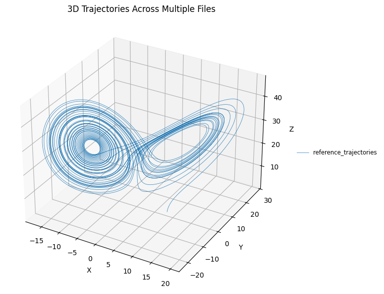
First, let’s take a look at the 3D trajectory.

plot_3d_trajectories([reference_trajectories])

100%|██████████| 1/1 [00:00<00:00, 126.58it/s]

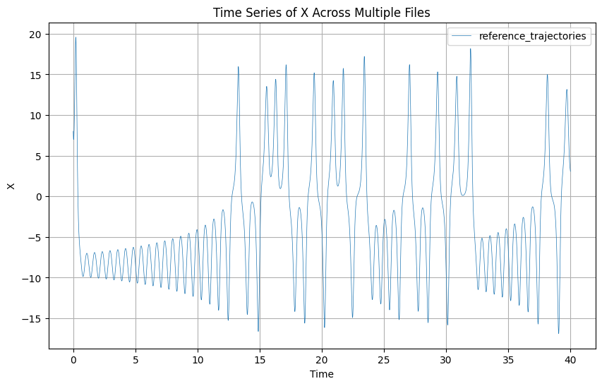
Now let’s look a the time series.

plot_trajectories(reference_trajectories)

100%|██████████| 1/1 [00:00<00:00, 85.19it/s]

Now that we saw what kind of results we can expect, let’s run with multiple cases. First, we will define the precisions that we want to try:

# Let's define the cases that we want to run:
cases = [5, 10, 20, 30, 45]

We could run all the cases sequentially using:

for precision in tqdm(cases):
    run_model(precision=precision)

but we will use joblib to run the cases in parallel:

n_jobs = -1
delayed_run_model = delayed(run_model)

# Run models in parallel
_ = Parallel(n_jobs=n_jobs)(
    delayed_run_model(precision=p) for p in cases
)

Results

After all cases have been executed, let’s look at the results:

# Find the case files
case_files = list(sorted(output_trajectories.parent.glob("case_trajectories_*")))
# Make 3D plot
plot_3d_trajectories(case_files + [reference_trajectories])

100%|██████████| 6/6 [00:00<00:00, 173.07it/s]

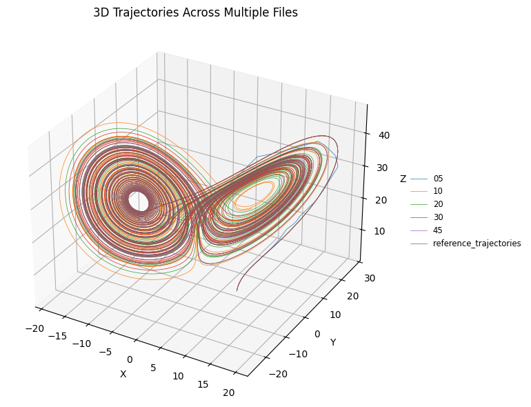
In this plot we can see that the run that uses only 5 bits for the coordinate quickly diverges, but it is hard to grasp where the other cases diverte. Let’s try with the time-series.

plot_trajectories(case_files + [reference_trajectories])

100%|██████████| 6/6 [00:00<00:00, 139.76it/s]

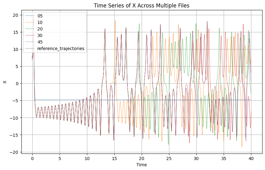
Here, it is easier to see that as we saw before the case with only 5 bits quickly diverges. For the other cases, even if it was not clear at the previous case, we can see that the lower the precision the sooner the trajectories diverge from the reference path, something that matches what was expected when simulating a chaotic system.

Great, feel free to play with the example.

Finally, it is recomended to clean the temporary directory and return to the original folder.

temp_dir.cleanup()
os.chdir(original_cwd)